3.1 Overview
In this paper, the inputs are genus 0 3D polyhedral models that consist of 1-ring structure triangular meshes. Our work is closest in spirit to Gregory et al.’s [3] work and to Alexa’s work [4]. Our overall system structure is similar to their theme. However, we present novel techniques in our design. The main procedures of our design are listed below:
l Selection of Vertex Pairs and Decomposition into Morphing Patches: For given two 3D polyhedral models, animators select corresponding vertices on each polyhedron to define correspondences of regions and points in both models. The algorithm automatically partitions the surface of each polyhedron into the same number of morphing patches by computing a shortest path between the selected vertices. The above is corresponding to the high-level control of morphs in our design.
l 3D-to-2D Embedding: Each 3D morphing patch is mapped onto a 2D regular polygon by the proposed relaxation method.
l Aligning Feature Vertices: The interior vertices in the regular 2D polygons are matched by using a foldover-free warping technique. Users can specify extra feature vertices to have a better control over correspondence. This design corresponds to the lower-level control of morphs.
l Merging, Re-meshing and Interpolation: The algorithm merges the topological connectivity of morphing patches in the regular 2D polygon. Inserting additional edges retriangulates the regions in the merged regular 2D polygon. This step reconstructs the facets for the new morphing patch, i.e., a common interpolation mesh. Finally, we compute exact interpolation across the common interpolation meshes.
3.2
Specifying Corresponding Morphing Patches
Given
two polyhedra A and B, animators interactively design
correspondence by partitioning each polyhedron into the same number of regions
called morphing patches. Each pair of morphing patches is denoted as (
![]() ,
,
![]() ), where
), where
![]() is the corresponding patch index.
To define each pair of (
is the corresponding patch index.
To define each pair of (
![]() ,
,
![]() ), animators must specify the same number of vertices (i.e., called extreme
vertices [3]), too. These selected vertices also form corresponding
point pairs in both models. The boundary of a morphing patch consists of several
consecutive chains. Each chain is obtained by computing a shortest path between
two consecutive selected vertices. Animators can partition two input polyhedra
into arbitrary number of morphing patches, but each patch cannot cross or
overlap the other patches. Once the models are partitioned into several
corresponding morphing patches, the next is to compute the correspondence of
interior vertices of (
), animators must specify the same number of vertices (i.e., called extreme
vertices [3]), too. These selected vertices also form corresponding
point pairs in both models. The boundary of a morphing patch consists of several
consecutive chains. Each chain is obtained by computing a shortest path between
two consecutive selected vertices. Animators can partition two input polyhedra
into arbitrary number of morphing patches, but each patch cannot cross or
overlap the other patches. Once the models are partitioned into several
corresponding morphing patches, the next is to compute the correspondence of
interior vertices of (
![]() ,
,
![]() ).
).
3.3
Embedding 3D Morphing Patches on Regular 2D Polygons
In the
following, we will first describe the basic idea of the proposed relaxation
method to compute 3D-to-2D embeddings. This initial approach requires several
iterations to be finished. It can be computationally expensive. Next, we propose
to solve the linear system of our relaxation method. In this manner, the
embedding can be computed very fast.
Given a pair
of 3D morphing patches (
![]() ,
,
![]() ) defined by n extreme vertices, we embed each on an n-side
regular 2D polygon called Di (
) defined by n extreme vertices, we embed each on an n-side
regular 2D polygon called Di (
![]() ,
,
![]() ) by a relaxation method. Each n-regular polygon is inscribed in the unit
circle and its center is at (0, 0). The relaxation algorithm consists of three
steps. First, the extreme vertices of the morphing patches are mapped to the
vertices of Di. Next, each chain of the morphing patch is
mapped to an edge of Di. We need to find the 2D coordinates of
non-extreme vertices along each chain. The 2D coordinates of these non-extreme
vertices are interpolated based on the arc length of the chain. Third, we
compute a 2D mapping for the interior vertices of
) by a relaxation method. Each n-regular polygon is inscribed in the unit
circle and its center is at (0, 0). The relaxation algorithm consists of three
steps. First, the extreme vertices of the morphing patches are mapped to the
vertices of Di. Next, each chain of the morphing patch is
mapped to an edge of Di. We need to find the 2D coordinates of
non-extreme vertices along each chain. The 2D coordinates of these non-extreme
vertices are interpolated based on the arc length of the chain. Third, we
compute a 2D mapping for the interior vertices of
![]() and
and
![]() by initially mapping them to the center position (0,0). Then, these vertices
are moved step by step by the following relaxation equation and this process
will continue until all the interior points are stable, i.e., not moved.
by initially mapping them to the center position (0,0). Then, these vertices
are moved step by step by the following relaxation equation and this process
will continue until all the interior points are stable, i.e., not moved.
 (1).
(1).
In equation (1), there are several parameters defined as follows:
l
![]() is an interior vertex and its
initial position is at (0,0). It represents the 2D mapping of a 3D vertex Pi
on a morphing patch.
is an interior vertex and its
initial position is at (0,0). It represents the 2D mapping of a 3D vertex Pi
on a morphing patch.
l
![]() is a new position of
is a new position of
![]() according to equation (1).
according to equation (1).
l
![]() is a 2D mapping of Pj.
Pj is one of Pi’s neighbors and
is a 2D mapping of Pj.
Pj is one of Pi’s neighbors and
![]() is the number of neighbors of Pi
in 3D.
is the number of neighbors of Pi
in 3D.
l
![]() is a pulling weight for
is a pulling weight for
![]() , and
, and
![]() controls the moving speed and its value is between 0 and 1.
controls the moving speed and its value is between 0 and 1.
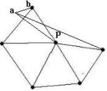
We attempt to
compute a good embedding which preserves the aspect ratio of the original
triangle versus the mapped triangle and does not cause too much distortion To
determine
![]() , our idea is similar to Kanai et al.’s [10] weight formula used in their
harmonic mapping. However, we use a different and a simpler formula. For
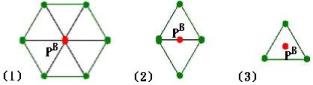
example, in Figure 1,
, our idea is similar to Kanai et al.’s [10] weight formula used in their
harmonic mapping. However, we use a different and a simpler formula. For
example, in Figure 1,
![]() is labeled 0 and the weight of a
is labeled 0 and the weight of a
![]() labeled by 2 is computed by the
following equation:
labeled by 2 is computed by the
following equation:
![]() (2)
(2)
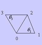
Fig. 1. The definition of a pulling weight
In
equation (2),
![]() is the angle between
is the angle between
![]() and
and
![]() and
and
![]() is the angle between
is the angle between
![]() and
and
![]() . These correspond to 3D edges of a morphing patch. In this manner, all
. These correspond to 3D edges of a morphing patch. In this manner, all
![]() can be computed. In equation (2),
we can imagine that the whole system is a spring system. During iterations,
can be computed. In equation (2),
we can imagine that the whole system is a spring system. During iterations,
![]() is pulled by several springs
connecting to all its neighbors
is pulled by several springs
connecting to all its neighbors
![]() . The idea behind the equation (2) is
that long edges subtending to big angles are given relatively small spring
constants compared with short edges that subtend to small angles. Based
on the equation (1), we can use iteration methods to find all
. The idea behind the equation (2) is
that long edges subtending to big angles are given relatively small spring
constants compared with short edges that subtend to small angles. Based
on the equation (1), we can use iteration methods to find all
![]() and terminate iteration when all
and terminate iteration when all
![]() are stable. However, in this
manner, the computation time is not predictable and could be expensive.
Therefore, we will not find
are stable. However, in this
manner, the computation time is not predictable and could be expensive.
Therefore, we will not find
![]() by iteration method and will solve
it by the following manner.
by iteration method and will solve
it by the following manner.
Using
equation (1), as
![]() is stable, ideally,
is stable, ideally,
![]() . Thus, we will have the following.
. Thus, we will have the following.
 =>
(3)
=>
(3)
Therefore,
assume the number of
![]() is N, we can have the
following linear
system for the proposed relaxation method.
is N, we can have the
following linear
system for the proposed relaxation method.
![]()
![]()
(4)
Let
 and
and
![]() , the above linear system can be represented as the following form:
, the above linear system can be represented as the following form:
![]()
![]()
![]()
![]() (5)
(5)
This
linear system is not singular, so that it has a unique solution. Furthermore,
for each
![]() , the number of its neighbors is small compared to N. Therefore it is a
sparse system and can be solved efficiently by using numerical method.
, the number of its neighbors is small compared to N. Therefore it is a
sparse system and can be solved efficiently by using numerical method.
3.4
Aligning the Features and Foldover-Free Warping
Given
a pair of morphing patches (
![]() ,
,
![]() ),
),
![]() are their corresponding 2D embeddings. Their extreme vertices are automatically
aligned by user specification. Using this initial correspondence, we could
directly overlay two embeddings to get a merged embedding for morphing. For
example in Figure 2 (a), we select a corresponding morphing patch on two given
models and the number of extreme vertices is five. There are two extra vertex
pairs
are their corresponding 2D embeddings. Their extreme vertices are automatically
aligned by user specification. Using this initial correspondence, we could
directly overlay two embeddings to get a merged embedding for morphing. For
example in Figure 2 (a), we select a corresponding morphing patch on two given
models and the number of extreme vertices is five. There are two extra vertex
pairs
![]() and
and
![]() shown in both models, respectively. These extra vertices represent eye corners.
In Figure 2(b), we show both
shown in both models, respectively. These extra vertices represent eye corners.
In Figure 2(b), we show both
![]() after embedding. It is obvious to
see that vertex pairs
after embedding. It is obvious to
see that vertex pairs
![]() and
and
![]() do not align if we directly overlay
do not align if we directly overlay
![]() . Therefore, to compute better correspondence, we usually require animators to
specify several extra corresponding features such as vertex pairs
. Therefore, to compute better correspondence, we usually require animators to
specify several extra corresponding features such as vertex pairs
![]() and
and
![]() on both
on both
![]() . Then we employ a foldover-free warping function to align
. Then we employ a foldover-free warping function to align
![]() and
and
![]() . Non-feature points will be automatically moved by the warping function, too.
Like [5], to minimize distortion due to warping, we first move these extra
corresponding feature points linearly to the point halfway between them and then
perform warping.
. Non-feature points will be automatically moved by the warping function, too.
Like [5], to minimize distortion due to warping, we first move these extra
corresponding feature points linearly to the point halfway between them and then
perform warping.
Our warping is
simply computed as a weighted sum of radial basis function (RBF). Suppose there
are n extra feature pairs. Since
![]() are both in 2D, the radial function R consists of two components
are both in 2D, the radial function R consists of two components
![]() , where each component has the following form.
, where each component has the following form.
![]() , j = 1,2
(6)
, j = 1,2
(6)
In
equation (6),
![]() are coefficients to be computed, g is the radial function and
are coefficients to be computed, g is the radial function and
![]() is a feature point.
For each given p, we compute its new position by
is a feature point.
For each given p, we compute its new position by
![]() using equation (6). In total, there are 2n coefficients to compute. In current
implementation, the radial basis function we use is a Gaussian function:
using equation (6). In total, there are 2n coefficients to compute. In current
implementation, the radial basis function we use is a Gaussian function:
 (7)
(7)
In
equation (7), the variance
![]() controls the degree of locality of
the transformation. In Figure 2 (c), we show
controls the degree of locality of
the transformation. In Figure 2 (c), we show
![]() with warping by two extra feature
points. This result is better than that of Figure 2(b). Therefore, we can
overlay them now to get a merged embedding for morphing. Sometimes, the warping
can lead to fold-over (self-intersections) on
with warping by two extra feature
points. This result is better than that of Figure 2(b). Therefore, we can
overlay them now to get a merged embedding for morphing. Sometimes, the warping
can lead to fold-over (self-intersections) on
![]() . We need foldover-free embeddings. To solve foldover, we first check if
self-intersections occur on
. We need foldover-free embeddings. To solve foldover, we first check if
self-intersections occur on
![]() after warping. If
self-intersections occur, we simply iterate equation (1) instead of solving
equation (5). Usually, it requires a few iterations and self-intersections will
not occur. In the following, we show how to check if self-intersections occur.
after warping. If
self-intersections occur, we simply iterate equation (1) instead of solving
equation (5). Usually, it requires a few iterations and self-intersections will
not occur. In the following, we show how to check if self-intersections occur.
Our inputs are
genus 0 3D polyhedral models with 1-ring structure. Therefore, if there is no
self-intersection on both
![]() , each interior point of both embeddings must have a complete 1-ring structure
in 2D. If any interior point of an embedding has an incomplete 1-ring structure,
the self-intersection occurs. To check if a point has a complete 1-ring
structure, we compute the following:
, each interior point of both embeddings must have a complete 1-ring structure
in 2D. If any interior point of an embedding has an incomplete 1-ring structure,
the self-intersection occurs. To check if a point has a complete 1-ring
structure, we compute the following:
![]() (
(
![]() : the right-hand vector
cross product)
: the right-hand vector
cross product)
![]() (8)
(8)
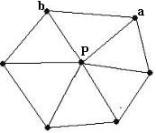
In equation (8), we need to check all nodes at p’s 1-ring structure. If any violation (i.e., M <=0) occurs, it is an incomplete ring structure in 2D. Note that the vertices of a triangle are in counterclockwise order. Figure 3 is used to illustrate the equation (8). In Figure 3 (a), before embedding, P (i.e., p’s corresponding vertex in 3D) has a complete 1-ring structure. After embedding and warping, a self-intersection occurs as shown in Figure 3 (b). In this case, we simply check all nodes at p’s 1-ring structure and find (a, b) violates equation (8).
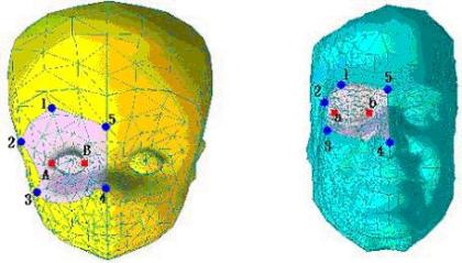
(a) The user picks five extreme vertices (i.e., blue dots) and two extra feature vertices (i.e., red dots).
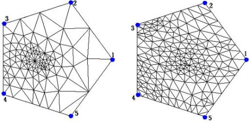
(b) Embeddings without warping.
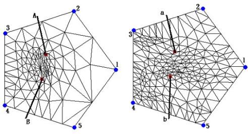
(c) Embedding with warping by two extra features (i.e., red dots).
Figure 2. Embedding and warping.
(a)
 (b)
(b)
Figure
3 (a) prior to embedding and warping,
![]() has a complete 1-ring structure in
3D and (b)
has a complete 1-ring structure in
3D and (b)
![]() has an incomplete 1-ring structure
in 2D after embedding and warping.
has an incomplete 1-ring structure
in 2D after embedding and warping.
3.5
Efficient Local Merging
Given two
embeddings
![]() , we merge them to produce a common embedding that contains the faces, edges and
vertices. The complexity of a brute-force merging algorithm is
, we merge them to produce a common embedding that contains the faces, edges and
vertices. The complexity of a brute-force merging algorithm is
![]() +k),where n is the number of edges and k is the number of
intersections. This naïve approach globally checks all edges to find the
possible intersections. We present a novel method for checking edges locally and
efficiently computing the intersections. The complexity of the proposed method
is
+k),where n is the number of edges and k is the number of
intersections. This naïve approach globally checks all edges to find the
possible intersections. We present a novel method for checking edges locally and
efficiently computing the intersections. The complexity of the proposed method
is
![]() . Additionally, to efficiently implement our method, a lookup table is created.
. Additionally, to efficiently implement our method, a lookup table is created.
3.5.1
The Classification of the Corresponding Positions
The merging
algorithm wants to overlay each edge
![]()
![]() on
on
![]() , where S and E represent the starting and ending points of a
given edge. Since the correspondence of each extreme vertex has been established
before embedding by animators, we perform the overlay starting from a
, where S and E represent the starting and ending points of a
given edge. Since the correspondence of each extreme vertex has been established
before embedding by animators, we perform the overlay starting from a
![]()
![]() , where
, where
![]() is an extreme vertex. Since
is an extreme vertex. Since
![]() is a connected planar graph, we can
traverse all edges starting from
is a connected planar graph, we can
traverse all edges starting from
![]() and overlay them on
and overlay them on
![]() edge by edge. We can imagine that
an edge
edge by edge. We can imagine that
an edge
![]() consists of an infinite number of points. As we overlay this edge on
consists of an infinite number of points. As we overlay this edge on
![]() , the corresponding positions of these points have three kinds on
, the corresponding positions of these points have three kinds on
![]() as illustrated in Figure 4. These
three possibilities are:
as illustrated in Figure 4. These
three possibilities are:
1.
Some point
![]() (i.e.,
(i.e.,
![]()
![]() ) falls on a vertex
) falls on a vertex
![]() of a triangle
of a triangle
![]()
![]() .
.
2.
Some point
![]() falls on an edge
falls on an edge
![]() of a triangle
of a triangle
![]()
![]() .
.
3.
Some point
![]() falls on the interior of a triangle
falls on the interior of a triangle
![]()
![]() .
.
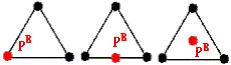
Figure 4. There are three kinds of
corresponding positions (i.e., red dot) on
![]() .
.
When an edge
![]() (for simplicity,
(for simplicity,
![]() is interchanged with
is interchanged with
![]() ) is overlaid on
) is overlaid on
![]() , this edge can be split into several line segments
, this edge can be split into several line segments
![]() by a triangle
by a triangle
![]()
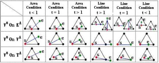
![]() . The relationship between
. The relationship between
![]() and
and
![]() can be classified into eighteen
kinds of cases (as shown in Figure 5). For example in Figure 6, the edge
can be classified into eighteen
kinds of cases (as shown in Figure 5). For example in Figure 6, the edge
![]() could be split into the following
cases (i.e., according to Figure 5) 15-2-2-6-9-2-2-3, 14-15-2-6-9-2-2-3, or
other sequences. But the former splitting sequence generates the minimum number
of new points on
could be split into the following
cases (i.e., according to Figure 5) 15-2-2-6-9-2-2-3, 14-15-2-6-9-2-2-3, or
other sequences. But the former splitting sequence generates the minimum number
of new points on
![]() . We shall call such splitting as the optimal splitting.
. We shall call such splitting as the optimal splitting.
Figure
5. The relationship between a line segment
![]() and
and
![]() can be classified into eighteen kinds of cases. The left-most column is
classified based on Figure 4.
can be classified into eighteen kinds of cases. The left-most column is
classified based on Figure 4.
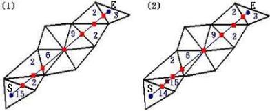
Figure
6. (a) The optimal splitting generates nine new points on
![]() . (b) The
non-optimal splitting generates ten new points on
. (b) The
non-optimal splitting generates ten new points on
![]() . In (a) and
(b), the label on each point is made according to Figure 5.
. In (a) and
(b), the label on each point is made according to Figure 5.
3.5.2 Structures of Minimal Contour Coverage (SMCC)
Whichever a
new point generated by the optimal splitting can be found with the help of
structures of minimal contour coverage (SMCC) on
![]() . Based on the classification in Figure 4, there are three kinds of SMCC for the
corresponding position (Figure 7) defined in the following.
. Based on the classification in Figure 4, there are three kinds of SMCC for the
corresponding position (Figure 7) defined in the following.
1.
For some point
![]() falls on
falls on
![]() ,
,
![]() ’s SMCC is
’s SMCC is
![]() ’s 1-ring structure.
’s 1-ring structure.
2.
For some point
![]() falls on
falls on
![]() , its SMCC is a 4-sided polygon containing
, its SMCC is a 4-sided polygon containing
![]() .
.
1.
For some point
![]() falls on
falls on
![]() , its SMCC is a triangle
, its SMCC is a triangle
![]() .
.
In above,
![]() ,
,
![]() and
and
![]() are all defined in Figure 4.
are all defined in Figure 4.
Figure
7. There are three kinds of SMCC for
![]() on
on
![]() : (1) 1-ring, (2) 4-sided polygon and (3) a triangle.
: (1) 1-ring, (2) 4-sided polygon and (3) a triangle.
Assume the
starting point
![]() of an edge
of an edge
![]() has established its SMCC on
has established its SMCC on
![]() . If
. If
![]() could generate new intersection
points with some edges
could generate new intersection
points with some edges
![]() outside S’s SMCC,
outside S’s SMCC,
![]() must generate a new intersection
point with S’s SMCC. To the contrary, if
must generate a new intersection
point with S’s SMCC. To the contrary, if
![]() does not intersect with S’s
SMCC, it also will not intersect with other edges
does not intersect with S’s
SMCC, it also will not intersect with other edges
![]() outside S’s SMCC (as shown
in Figure 8). So the merging can be done locally with S’s SMCC.
outside S’s SMCC (as shown
in Figure 8). So the merging can be done locally with S’s SMCC.
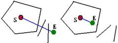
Figure 8. The merging can be locally done with S’s SMCC.
The local
merging can be further classified into two kinds of the merging conditions. One
is called area condition at which the local case
![]() is not co-incident with any
imaginary line that links s with the contour vertex of SMCC. If
is not co-incident with any
imaginary line that links s with the contour vertex of SMCC. If
![]() is co-incident with any imaginary
line, this is called line condition (as shown in Figure 9). The determination of
the local merging condition is evaluated by the following:
is co-incident with any imaginary
line, this is called line condition (as shown in Figure 9). The determination of
the local merging condition is evaluated by the following:
M
=
![]()
![]()
![]() , N
=
, N
=
![]()
![]()
![]() , where
, where
![]() ,
,
![]() and
and
![]()
![]() .
.
 (9)
(9)
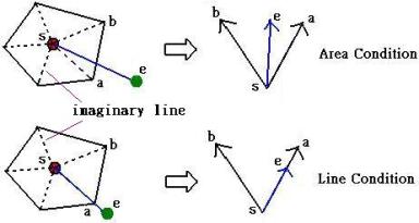
Figure 9. There are two kinds of the local merging conditions.
Based on the
above classifications, we can use different formulas (i.e., equation (10) and
(11)) to determine whether
![]() intersects with S’s SMCC
or not. The results of equation
(10) and (11) lead to different conditions as showed in Figure 10.
intersects with S’s SMCC
or not. The results of equation
(10) and (11) lead to different conditions as showed in Figure 10.
1. Area Condition:
Let
![]() , and suppose V on the
, and suppose V on the
![]() ,
,
![]()
![]()
Then
![]()
![]()
![]()
![]() Let
Let
![]()
![]()
![]() (10)
(10)
2. Line Condition: (assume co-incident with
![]() )
)
![]()
![]()
![]() (11)
(11)
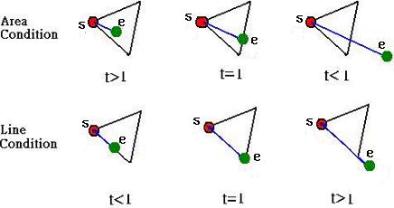
(a)
The results of the equation (10) and (11).
(b) Local merging condition table.
Figure 10. Classifications of local merging conditions
Based on the analysis of Figure 10 (b), we can replace Figure 5 with Figure 10 (b). Figure 10 (b) can provide us a lookup table to efficiently implement our merging algorithm.
Our merging
algorithm needs to establish the SMCC structure prior to proceeding the local
merging. In Figure 7, we have demonstrated how to find a SMCC structure. In our
design, once a new intersection occurs, we will establish its SMCC immediately
for further potential merging. For example, in Figure 11, an edge
![]() and A’s SMCC has been
created using Figure 7. Using Figure 10 (b), we find
and A’s SMCC has been
created using Figure 7. Using Figure 10 (b), we find
![]() intersects with A’s SMCC
at C. Next, we create C’s SMCC using Figure 7 again. Again, with
the help of Figure 10 (b), the edge
intersects with A’s SMCC
at C. Next, we create C’s SMCC using Figure 7 again. Again, with
the help of Figure 10 (b), the edge
![]() intersects with C’s SMCC
at D. In this manner, we repeat the above steps until we reach at B.
Of course, we need to create B’s SMCC, since B could be the
starting point of the other edge (i.e., not yet overlaid) from
intersects with C’s SMCC
at D. In this manner, we repeat the above steps until we reach at B.
Of course, we need to create B’s SMCC, since B could be the
starting point of the other edge (i.e., not yet overlaid) from
![]() . Finally, we recall in Section 3.5.1 that we start the local merging from an
extreme vertex. The SMCC of an extreme vertex is its 1-ring structure. Given two
embeddings
. Finally, we recall in Section 3.5.1 that we start the local merging from an
extreme vertex. The SMCC of an extreme vertex is its 1-ring structure. Given two
embeddings
![]() in Figure 12, we show a complete
sequence of overlaying
in Figure 12, we show a complete
sequence of overlaying
![]() on
on
![]() by the proposed method.
by the proposed method.
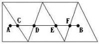
Figure 11. The merging of
![]() can be completed step by step.
can be completed step by step.
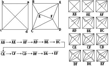
Figure 12. An example of merging is completed step by step by our algorithm.
3.6
Re-triangulate the Merged Embeddings
Once the
merging is completed, we produce a non-triangulated planar graph called
![]() . In order to re-triangulate
. In order to re-triangulate
![]() , we need to insert additional edges to re-triangulate
, we need to insert additional edges to re-triangulate
![]() . For simplicity, our approach is very straightforward and is described as
follows. For each point
. For simplicity, our approach is very straightforward and is described as
follows. For each point
![]() on
on
![]() , the algorithm must connect the neighboring points of
, the algorithm must connect the neighboring points of
![]() to establish its 1-ring cyclic
structure. Our design principle (as shown in Figure 13) is that the inserted
edge (i.e., red line in Figure 13) connecting the neighboring points is not
allowed to generate any new intersection point with other existing edges (i.e.,
green lines). It is very easy to check if an inserted edge intersects with other
edges or not. We can easily adapt the equation (10) for this purpose.
to establish its 1-ring cyclic
structure. Our design principle (as shown in Figure 13) is that the inserted
edge (i.e., red line in Figure 13) connecting the neighboring points is not
allowed to generate any new intersection point with other existing edges (i.e.,
green lines). It is very easy to check if an inserted edge intersects with other
edges or not. We can easily adapt the equation (10) for this purpose.
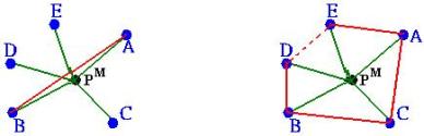
Figure 13. (a)
The inserted
![]() is not legal and (b)
is not legal and (b)
![]() ’s 1-ring cyclic structure is established by inserting several legal edges.
’s 1-ring cyclic structure is established by inserting several legal edges.
3.7
Reconstructing the Source Models and Interpolation
Once we finish
the preceding steps, we have established a complete correspondence between two
models. Our merging algorithm produces new points in 2D due to intersections.
For these new points, we need to find its corresponding 3D points in both
models. We first compute the barycentric representation of a new point in the
basis of three old points in 2D. Then, the barycentric representation is used to
interpolate positions of these three old points in 3D. These old points are
referred to the original vertices on the input models. In this manner we find 3D
position of a new point. Similarly, for a new point, we can interpolate its
other attributes such as color and texture coordinates if required.
Once the above step is finished, the morphing sequence can be easily generated by linearly moving each vertex from its position in model A to the corresponding position in model B in term of time t. Other authors mentioned this kind of linear interpolation can produces satisfying results in most cases. However, in some special case, the self-intersections can occur. Gregory et al. [3] propose the user-specified morphing trajectory by the cubic spline curves for an alternative to linear interpolation. This simple alternative can be included in near future.