 |
|
| (left) (right) | |
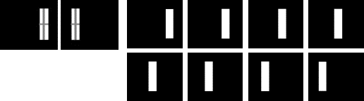
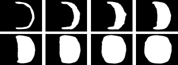
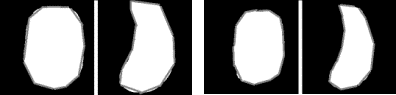
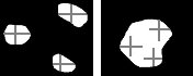
| Figure 8. Interpolation between two synthetic contours with a large offset. On the left side, two feature lines are marked on each slice. |
Experiments
In this
section, many synthesized images that were used or similar to those used in
previous studies were used to evaluate the proposed interpolation method. In the
most following illustrations, the left side of figures shows the original two
input contour objects and specified feature lines. The right side of figures
shows a sequence of interpolation using the proposed method.
Interpolation
using a pair of synthetic contours is illustrated in Figure 8 (left). Lee et
al. [12] showed that if there is no prior alignment between these two input
images, shape-based interpolation couldn’t perform well. The shape-based
method creates a bad interpolation, where there is no contour in the
interpolated image. In contrast, the proposed method yields better interpolation
as shown in Figure 8 (right). In fact, the proposed method employs features to
automatically achieving the task of object centralization used in [12].
Additionally, in Figure 4 shown in previous section, the source image contains a
small ring, while target image contains a large one with a large offset. This
case was not handled well by morphology-based scheme [10]. In contrast, the
proposed method performs very well.
|
|
| (left) (right) | |
| Figure 8. Interpolation between two synthetic contours with a large offset. On the left side, two feature lines are marked on each slice. |
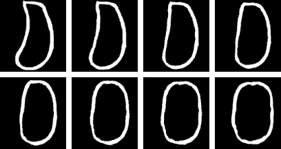
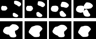
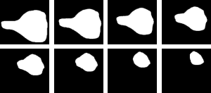
Both
Figures 9 and 10 were tested in [6]. Lin et
al. [6] termed Figure 9 a “moderate” concave case and Figure 10 an
“extreme” concave case. Their approach employed a very computationally
intensive method to distort one contour to like another one. This approach can
yield satisfactory results for the moderate concave case, but not for the
extreme concave case. Using the simpler proposed scheme, the shapes of
intermediate contour change smoothly between two different shape contours for
both “moderate” and “extreme” concave cases. In these two examples, the
shapes pf two given contours do not change globally. The left portion of figures
is either shrinking or enlarging. Therefore, we cannot simply place two cross
lines like Figure 8 on these two examples. Alternatively, we place corresponding
feature lines along the boundaries of two given contours. In this manner, these
features can effectively control the change of shapes.
 |
 |
| (left) | (right) |
| Figure 9. A “moderate” concave case [6]. | |
 |
 |
| (left) | (right) |
|
Figure
10. An “extreme” concave case [6]. |
|
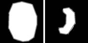
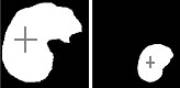
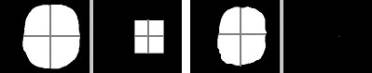
Many
previous studies suggested to apply object centralization to have one object
enclosed by another one before interpolation [16,17,18]. Sun et
al. pointed out that this conventional centralization (i.e., aligning the
centroids of the two objects) sometimes fail when the objects are concave like
Figure 11 (left) and 12. To solve this issue, Sun et
al. [11] iteratively employed object centralization and object enlargement
to ensure that object enclosure can occur. After interpolation, this approach
requires contour shrinking by means of erosion to compensate the effect of
object enlargement. Furthermore, this process cannot always guarantee object
enclosure even when the enlarging factor becomes extremely large [11]. The whole
process seems not very efficient with respect to computational complexity. In
this respect, our proposed scheme seems more practical than this approach.
Figure 11 (right) shows a sequence of interpolated results using the proposed
scheme.
 |
 |
| (left) | (right) |
| Figure 11. Object enclosure does not occur after applying conventional centralization on two concave objects [11]. | |
 |
| Figure 12. Overlapping of concave objects after centroid alignment cannot guarantee to achieve object enclosure [11]. |
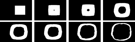
The next two examples were evaluated in [10]. Figure 13 is a set of ring-like objects with no overlapping area and Figure 14 illustrates the interpolation between a hollow object and a solid object. In both cases, we need to generate negative objects due to holes. Figure 14 needs to generate a pseudo negative hole. Then, we separately interpolated positive and negative object pairs and then blended them like our previous work [12]. Guo et al. [10] reported that both cases are not handled well by the original shape-based method. Shape-based method simply interpolates distance code for the whole image. Guo et al. [10] also pointed out that [6] fails to deal with Figure 14, but this dynamic elastic method is very computationally intensive. However, our results show the proposed scheme yields very satisfactory results in both examples.
(c)
Interpolation Figure
13. Interpolation for a set of ring-like objects [12]
(a) positive object pair
(b) negative object pair
 |
| (a) positive object pair (b) negative object pair |
 |
|
(c)
Interpolation |
|
Figure
14. Interpolation between a hollow object and a solid object [12]. |
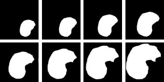
Branching
examples like Figure 15 have been widely evaluated [6,7,10,11, 12]. The proposed
scheme can successfully deal with Figure 15. Like [12], we first independently
interpolate three positive object pairs and then unite these three interpolated
results together to accomplish interpolation. Multiple objects may exist on two
input slices. In this situation, we will also employ our previous method [12] to
solve matching problem first and then use similar procedures to perform
interpolation. In this experiment, each positive object pair has two different
pairs of feature lines. These features effectively control where two positive
objects are merged. In other words, the user can fully control interpolation
with features.
 |
 |
|
(left) |
(right) |
|
Figure 15. Branching case [6,7,10,11,12]. |
|
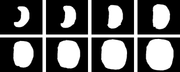
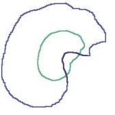
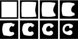
Figure
16 is called heavy invagination case (i.e., abrupt change in shape) in [11].
This case was not handled well by a morphology-based scheme [11,10]. From our
results, it is clear that the proposed scheme can handle invagination case well,
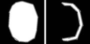
too. Lee et al. [12] cannot solve a
narrow concavity problem like Figure 17. In this example, there are two objects
X0 and Xn+1 and the region
![]() is equal to X0. There is
a very narrow concavity (i.e., marked by A) in the object X0. In this
situation, using method presented in Lee et al. [12], the distance codes of region near B is greater than
those of region near to A. Therefore, unfortunately, this method can not ensure
Xn+1 to contract into the region near B in the course of
interpolation. In contrast, the proposed method also easily solve this problem
by placing several corresponding feature lines along the boundaries of both
objects as illustrated in Figure 17.
is equal to X0. There is
a very narrow concavity (i.e., marked by A) in the object X0. In this
situation, using method presented in Lee et al. [12], the distance codes of region near B is greater than
those of region near to A. Therefore, unfortunately, this method can not ensure
Xn+1 to contract into the region near B in the course of
interpolation. In contrast, the proposed method also easily solve this problem
by placing several corresponding feature lines along the boundaries of both
objects as illustrated in Figure 17.
 |
 |
| (left) | (right) |
|
Figure
16. The invagination case (abrupt change in shape) [11]. |
|
Figure
17. The narrow concavity case [12].

(left)
(right)
We have
evaluated the proposed scheme using a variety of examples that used in the
previous work. Since our method employs feature control to help shape-based
interpolation, the results such as Figure 4, 6, 8, 13, 14 and 15 are reasonable
and continuous and smoother than are obtained by the original shape-based
method. Additionally, with feature control, our method considers the global and
local change of shapes in two given objects, so the proposed method can handle
cases with complicated structure such as Figure 10, 11, 16 and 17, that cannot
be handled well by the other methods. With the concept of positive and negative
objects [12], our method can simply handle the hollow and branching cases by the
same procedures, so that the results can be obtained easily just merging all
intermediate objects using a blending order presented in our previous work [12].
In summary, from above examples with synthesized objects, the proposed method
handles different situations effectively.
performs
faster than non-optimized for all experiments. If multiple object pairs are
interpolated, we also list the number of features for each pair in this table
such as Figure 13 and 15. Our experiments were performed on the Intel Pentium
II, 233MHZ personal computer with 256 MB main memory. This table indicates that
the execution time is in proportion to the number of object pairs and feature
lines. Since we perform interpolation on the whole image, the execution cost is
in proportion to the image resolution, too. Observing all experiments, we can
know it is not necessary to perform interpolation in this manner. We can save
more computation cost as follows. For each object pair, we find the union of
their bounding boxes and we just need to perform the same interpolation
procedure to this union area like Figure 18. Additionally, we will only perform
distance transform on this area, too. In this manner, we can achieve identical
results but with lower computation cost as shown in Table 1, too. With this
minor change in our implementation, the executing performance is much improved.
Like Figure 3, the performance is even faster by about 4.8 times. The main
reason is that the union area of two bounding boxes is still not significant
(i.e., about 20%) in contrast to the whole image. In this situation, we can save
time for both distance transform and interpolation.
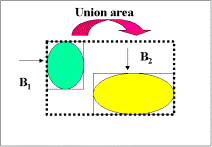
Figure 18. B1 and B2 are bounding boxes for two given objects and both distance transform and interpolation is performed only on the union area instead of the whole image to save computation cost.
|
|
Non-optimized |
Optimized |
Optimized
& Bounding Box |
No. features |
|
Fig 3 |
1.86 |
1.32 |
0.39 |
2 |
|
Fig 4 |
2.14 |
1.59 |
1.10 |
2 |
|
Fig 6 |
2.20 |
1.64 |
0.37 |
2 |
|
Fig 7 |
3.62 |
2.74 |
1.16 |
4 |
|
Fig 8 |
2.02 |
1.60 |
0.77 |
2 |
|
Fig 9 |
8.72 |
6.90 |
4.15 |
11 |
|
Fig 10 |
10.22 |
7.97 |
5.52 |
13 |
|
Fig 11 |
2.21 |
1.60 |
1.33 |
2 |
|
Fig 13 |
17.19 |
13.25 |
10.10 |
11 – 13 |
|
Fig 14 |
3.97 |
2.97 |
1.88 |
2 – 2 |
|
Fig 15 |
5.89 |
4.24 |
3.99 |
2 – 2 – 2 |
|
Fig 16 |
2.02 |
1.59 |
1.42 |
2 |
|
Fig 17 |
18.89 |
14.71 |
11.02 |
24 |
Table
1. Execution timing (in second) and the number of features for all experiments.